Logistic regression is a simple classification method which is widely used in the field of machine learning. Today we’re going to talk about how to train our own logistic regression model in Python to build a a binary classifier. We’ll use NumPy for matrix operations, SciPy for cost minimization, Matplotlib for data visualization and no machine learning tools or libraries whatsoever.
Problem & Dataset
We’ll be looking at another assignment from the machine learning course taught by Andrew Ng. Our objective in this problem is to estimate an applicant’s probability of admission into a university based on his/her results on two exams. Our dataset contains some historical data from previous applicants, which we’ll use as a training sample. Let’s read the dataset file and take a look at the first few examples:
1 | import numpy as np |
[[ 34.62365962  78.02469282   0.        ]
 [ 30.28671077  43.89499752   0.        ]
 [ 35.84740877  72.90219803   0.        ]
 [ 60.18259939  86.3085521    1.        ]
 [ 79.03273605  75.34437644   1.        ]]
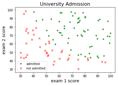
The first two columns correspond to the exam scores and the third column indicates whether the applicant has been admitted to the university. We can visualize this data using a scatter plot:
1 | fig, ax = plt.subplots() |

Hypothesis Function
Logistic regression is a linear model, which means that the decision boundary has to be a straight line. This can be achieved with a a simple hypothesis function in the following form:
$h_\theta(x) = g(\theta^Tx)$
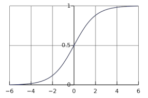
where $g$ is the sigmoid function which is defined as:
$g(z) = \dfrac{1}{1 + e^{-z}}$

Here’s the Python version of the sigmoid function:
1 | def sigmoid(z): |
The numeric output of the hypothesis function $h_\theta(x)$ corresponds to the model’s confidence in labeling the input:
- If the output is $0.5$, both classes are equally probable as far as the classifier is concerned.
- If the output is $1$, the classifier is 100% confident about class 1.
- If the output is $0$, the classifier is 100% confident about class 0.
In other words, the classifier labels the input based on whether $\theta^Tx$ is positive or negative. Of course this is based on the assumption that the treshold is selected as $0.5$.
Cost Function
In the training stage, we’ll try to minimize the cost function below:
$J(\theta) = \dfrac{1}{m}\sum\limits_{i=1}^{m}[-y^{(i)}log(h_\theta(x^{(i)})) - (1 - y^{(i)})log(1 - h_\theta(x^{(i)}))]$
Notice that this cost function penalizes the hypothesis according to its probability estimation error, as demonstrated below:
<br >
We can use the following Python function to compute this cost in our script:
1 | def cost(theta, X, y): |
Optimization Algorithm
We’re going to use the fmin_cg function from scipy.optimize to minimize our cost. fmin_cg needs the gradient of the cost function as well as the cost function itself. Here’s the formula for the cost gradient:
$\dfrac{\partial{J(\theta)}}{\partial{\theta_j}} = \dfrac{1}{m}\sum\limits_{i=1}^{m}(h_\theta(x^{(i)}) - y^{(i)})x^{(i)}_j$
where $m$ is the number of training examples.
And the Python version is:
1 | def cost_gradient(theta, X, y): |
If you’re not familiar with fmin_cg, it might be a good idea to check out my previous post and/or the official docs before proceeding to the next section.
Training Stage
The final thing we need to do before training our model is to add an additional first column to $x$, in order to account for the intercept term $\theta_0$:
1 | X = np.ones(shape=(x.shape[0], x.shape[1] + 1)) |
Finally we can train our logistic regression model:
1 | initial_theta = np.zeros(X.shape[1]) # set initial model parameters to zero |
Optimization terminated successfully.
         Current function value: 0.203498
         Iterations: 51
         Function evaluations: 122
         Gradient evaluations: 122
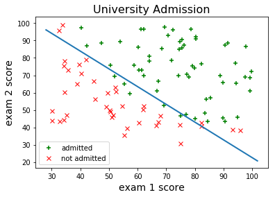
Now let’s plot the decision boundary of our optimized model:
1 | x_axis = np.array([min(X[:, 1]) - 2, max(X[:, 1]) + 2]) |

Looks pretty good. Let's also measure the training accuracy:
1 | predictions = np.zeros(len(y)) |
Training Accuracy = 89.0%Not bad at all. We would probably need something little more flexible than logistic regression if we wanted to come up with a more accurate classifier.
Prediction
Finally, here’s how we can predict the probability of admission for a student with arbitrary exam scores:
1 | probability = sigmoid(np.array([1, 45, 85]) @ theta) |
For a student with scores 45 and 85, we predict an admission probability of 0.776195474168If you’re still here, you should subscribe to get updates on my future articles.