Learning curves are very useful for analyzing the bias-variance characteristics of a machine learning model. In this post, I’m going to talk about how to make use of them in a case study of a regression problem. We’re going to start with a simple linear regression model and improve it as much as we can by taking advantage of learning curves.
Introduction to Learning Curves
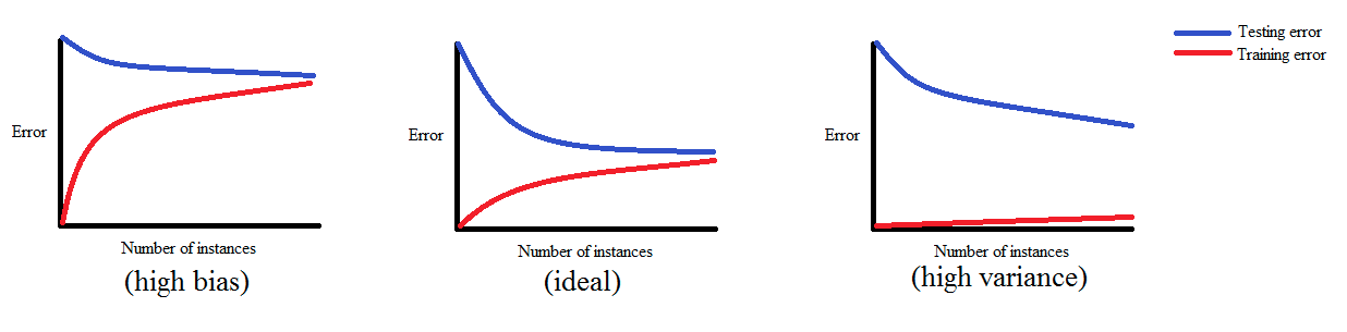
In a nutshell, learning curves show how the training and validation errors change with respect to the number of training examples used while training a machine learning model.
If a model is balanced, both errors converge to small values as the training sample size increases.
If a model has high bias, it ends up underfitting the data. As a result, both errors fail to decrease no matter how many examples there are in the training set.
If a model has high variance, it ends up overfitting the training data. In that case, increasing the training sample size decreases the training error but it fails to decrease the validation error.
The figure below demonstrates each of those cases:
Problem Definition and Dataset
After this incredibly brief introduction, let me introduce you to today’s problem where we’ll get to see learning curves in action. It’s another problem from Andrew Ng’s machine learning course, in which the objective is to predict the amount of water flowing out of a dam, given the change of water level in a reservoir.
The dataset file we’re about to read contains historical records on the change in water level and the amount of water flowing out of the dam. The reason that it’s a .mat file is because this problem is originally a MATLAB assignment. Fortunately, it’s pretty easy to load .mat files in Python using the loadmat function from SciPy. We’ll also need NumPy and Matplotlib for matrix operations and data visualization:
1 | import numpy as np |
The dataset is divided into three samples:
- The training sample consists of
x_trainandy_train. - The validation sample consists of
x_valandy_val. - The test sample consists of
x_testandy_test.
Notice that we have to explicitly convert the target variables (y_train, y_val and y_test) to one dimensional vectors, because they are stored as matrices inside the .mat file.
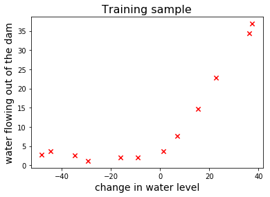
Let’s plot the training sample to see what it looks like:
1 | fig, ax = plt.subplots() |
The Game Plan
Alright, it’s time to come up with a strategy. First of all, it’s clear that there’s a nonlinear relationship between $x$ and $y$. Normally we would rule out any linear model because of that. However, we are going to begin by training a linear regression model so that we can see how the learning curves of a model with high bias look like.
Then we’ll train a polynomial regression model which is going to be much more flexible than linear regression. This will let us see the learning curves of a model with high variance.
Finally, we’ll add regularization to the existing polynomial regression model and see how a balanced model’s learning curves look like.
Linear Regression
I’ve already shown you in the previous post how to train a linear regression model using gradient descent. Before proceeding any further, I strongly encourage you to take a look at it if you don’t have at least a basic understanding of linear regression.
Here I’ll show you an easier way to train a linear regression model using an optimization function called fmin_cg from scipy.optimize. You can check out the detailed documentation here. The cool thing about this function is that it’s faster than gradient descent and also you don’t have to select a learning rate by trial and error.
fmin_cg needs a function that returns the cost and another one that returns the gradient of the cost for a given hypothesis. We have to pass those to fmin_cg as function arguments. Fortunately, we can reuse some code from the previous post:
- We can completely reuse the
costfunction because it’s independent of the optimization method that we use. - From the
gradient_descentfunction, we can borrow the part where the gradient of the cost function is evaluated.
So here’s (almost) all we need in order to train a linear regression model:
1 | def cost(theta, X, y): |
If you look at our cost function, there we evaluate the cross product of the feature matrix $X$ and the vector of model parameters $\theta$. Remember, this is only possible if the matrix dimensions match. Therefore we also need a tiny utility function to insert an additional first column of all ones to a raw feature matrix such as x_train.
1 | def insert_ones(x): |
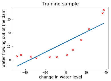
Now let’s train a linear regression model and plot the linear fit on top of the training sample:
1 | X_train = insert_ones(x_train) |
Learning Curves for Linear Regression
The above plot clearly shows that linear regression is not suitable for this task. Let’s also look at its learning curves and see if we can draw the same conclusion.
While plotting learning curves, we’re going to start with $2$ training examples and increase them one by one. In each iteration, we’ll train a model and evaluate the training error on the existing training sample, and the validation error on the whole validation sample:
1 | def learning_curves(X_train, y_train, X_val, y_val): |
In order to use this function, we have to resize x_val just like we did x_train:
1 | X_val = insert_ones(x_val) |
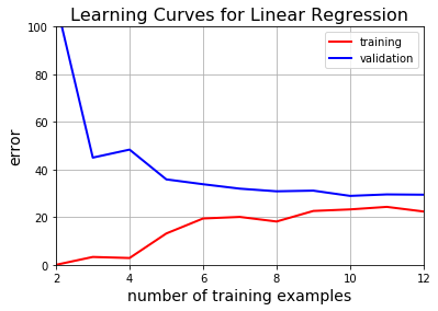
As expected, we were unable to sufficiently decrease either the training or the validation error.
Polynomial Regression
Now it’s time to introduce some nonlinearity with polynomial regression.
Feature Mapping
In order to train a polynomial regression model, the existing feature(s) have to be mapped to artificially generated polynomial features. Then the rest is pretty much the same drill.
In our case we only have a single feature $x_1$, the change in water level. Therefore we can simply compute the first several powers of $x_1$ to artificially obtain new polynomial features. Let’s create a simple function for this:
1 | def poly_features(x, degree): |
Now let’s generate new feature matrices for training, validation and test samples with 8 polynomial features in each:
1 | x_train_poly = poly_features(x_train, 8) |
Feature Normalization
Ok, we have our polynomial features but we also have a tiny little problem. If you take a closer look at one of the new matrices, you’ll see that the polynomial features are very imbalanced at the moment. For instance, let’s look at the first few rows of the x_train_poly matrix:
1 | print(x_train_poly[:4, :]) |
[[ -1.59367581e+01   2.53980260e+02  -4.04762197e+03   6.45059724e+04
   -1.02801608e+06   1.63832436e+07  -2.61095791e+08   4.16102047e+09]
 [ -2.91529792e+01   8.49896197e+02  -2.47770062e+04   7.22323546e+05
   -2.10578833e+07   6.13900035e+08  -1.78970150e+10   5.21751305e+11]
 [  3.61895486e+01   1.30968343e+03   4.73968522e+04   1.71527069e+06
    6.20748719e+07   2.24646160e+09   8.12984311e+10   2.94215353e+12]
 [  3.74921873e+01   1.40566411e+03   5.27014222e+04   1.97589159e+06
    7.40804977e+07   2.77743990e+09   1.04132297e+11   3.90414759e+12]]
As the polynomial degree increases, the values in the corresponding columns exponentially grow to the point where they differ by orders of magnitude.
The thing is, the cost function will generally converge much more slowly when the features are imbalanced like this. So we need to make sure that our features are on a similar scale before we begin to train our model. We’re going to do this in two steps:
- Subtract the mean value of each column from itself and make the new mean $0$.
- Divide the values in each column by their standard deviation and make the new standard deviation $1$.
It’s important that we use the mean and standard deviation values from the training sample while normalizing the validation and test samples.
1 | train_means = x_train_poly.mean(axis=0) |
Finally we can train our polynomial regression model by using our train_linear_regression function and plot the polynomial fit. Note that when the polynomial features are simply treated as independent features, training a polynomial regression model is no different than training a multivariate linear regression model:
1 | def plot_fit(min_x, max_x, means, stdevs, theta, degree): |
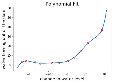
What do you think, seems pretty accurate right? Let’s take a look at the learning curves.
1 | plt.title("Learning Curves for Polynomial Regression", fontsize=16) |

Now that’s overfitting written all over it. Even though the training error is very low, the validation error miserably fails to converge.
It appears that we need something in between in terms of flexibility. Although we can’t make linear regression more flexible, we can decrease the flexibility of polynomial regression using regularization.
Regularized Polynomial Regression
Regularization lets us come up with simpler hypothesis functions that are less prone to overfitting. This is achieved by penalizing large $\theta$ values during the training stage.
Here’s the regularized cost function:
$J(\theta) = \dfrac{1}{2m}\Big(\sum\limits_{i=1}^{m}(h_\theta(x^{(i)}) - y^{(i)})^2\Big) +
\dfrac{\lambda}{2m}\Big(\sum\limits_{j=1}^{n}\theta_j^2\Big)$
And its gradient becomes:
$\dfrac{\partial J(\theta)}{\partial \theta_0} =
\dfrac{1}{m}\sum\limits_{i=1}^{m}(h_\theta(x^{(i)}) - y^{(i)})x_j^{(i)}
\quad \qquad \qquad \qquad for ,, j = 0$
$\dfrac{\partial J(\theta)}{\partial \theta_j} =
\Big(\dfrac{1}{m}\sum\limits_{i=1}^{m}(h_\theta(x^{(i)}) - y^{(i)})x_j^{(i)}\Big) + \dfrac{\lambda}{m}\theta_j
,,\quad \qquad for ,, j \geq 0$
Notice that we are not penalizing the intercept term $\theta_0.$ That’s because it doesn’t have anything to do with the model’s flexibility.
Of course we’ll need to reflect these changes to the corresponding Python implementations by introducing a regularization parameter lamb:
1 | def cost(theta, X, y, lamb=0): |
We also have to slightly modify train_linear_regression and learning_curves:
1 | def train_linear_regression(X, y, lamb=0): |
Alright we’re now ready to train a regularized polynomial regression model. Let’s set $\lambda = 1$ and plot our polynomial hypothesis on top of the training sample:
1 | theta = train_linear_regression(X_train_poly, y_train, 1) |
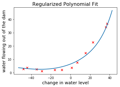
It is clear that this hypothesis is much less flexible than the unregularized one. Let’s plot the learning curves and observe its bias-variance tradeoff:
1 | plt.title("Learning Curves for Regularized Polynomial Regression", fontsize=16) |
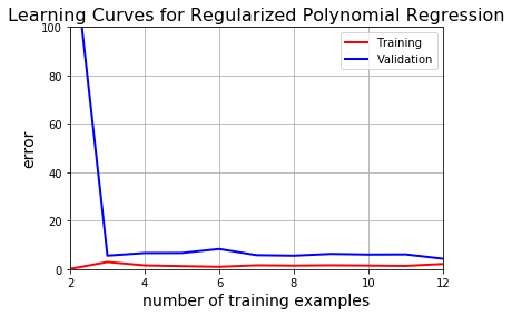
This is apparently the best model we’ve come up so far.
Choosing the Optimal Regularization Parameter
Although setting $\lambda = 1$ has significantly improved the unregularized model, we can do even better by optimizing $\lambda$ as well. Here’s how we’re going to do it:
- Select a set of $\lambda$ values to try out.
- Train a model for each $\lambda$ in the set.
- Find the $\lambda$ value that yields the minimum validation error.
1 | lambda_values = [0, 0.001, 0.003, 0.01, 0.03, 0.1, 0.3, 1, 3, 10]; |
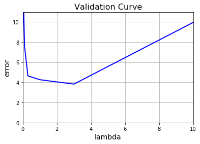
Looks like we’ve achieved the lowest validation error where $\lambda = 3$.
Evaluating Test Errors
It’s good practice to evaluate an optimized model’s accuracy on a separate test sample other than the training and validation samples. So let’s train our models once again and compare test errors:
1 | X_test = insert_ones(x_test) |
Test Error = 32.5057492449 | Linear Regression
Test Error = 17.2624144407 | Polynomial Regression
Test Error = 3.85988782246 | Regularized Polynomial Regression (at lambda = 3)
If you’re still here, you should subscribe to get updates on my future articles.