Hey everyone, welcome to my first blog post! This is going to be a walkthrough on training a simple linear regression model in Python. I’ll show you how to do it from scratch, without using any machine learning tools or libraries. We’ll only use NumPy and Matplotlib for matrix operations and data visualization.
Problem & Dataset
We’ll look at a regression problem from a very popular machine learning course taught by Andrew Ng. Our objective in this problem will be to train a model that accurately predicts the profits of a food truck.
The first column in our dataset file contains city populations and the second column contains food truck profits in each city, both in $10,000$s. Here are the first few training examples:
1 | 6.1101,17.592 |
We’re going to use this dataset as a training sample to build our model. Let’s begin by loading it:
1 | import numpy as np |
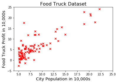
Both $x$ and $y$ are one dimensional arrays, because we have one feature (population) and one target variable (profit) in this problem. Therefore we can conveniently visualize our dataset using a scatter plot:
1 | fig, ax = plt.subplots() |
Hypothesis Function
Now we need to come up with a straight line which accurately represents the relationship between population and profit. This is called the hypothesis function and it’s formulated as:
$h_\theta(x) = \theta^Tx = \theta_0 + \theta_1x_1 + \theta_2x_2 + … + \theta_nx_n$
where $x$ corresponds to the feature matrix and $\theta$ corresponds to the vector of model parameters.
Since we have a single feature $x_1,$ we’ll only have two model parameters $\theta_0$ and $\theta_1$ in our hypothesis function:
$h_\theta(x) = \theta_0 + \theta_1x_1$
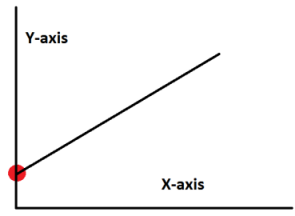
As you may have noticed, the number of model parameters is equal to the number of features plus $1$. That’s because each feature is weighted by a parameter to control its impact on the hypothesis $h_\theta(x)$. There is also an independent parameter $\theta_0$ called the intercept term, which defines the point where the hypothesis function intercepts the $y$-axis as demonstrated below:
The predictions of a hypothesis function can easily be evaluated in Python by computing the cross product of $x$ and $\theta^T.$ At the moment we have our $x$ and $y$ vectors but we don't have our model parameters yet. So let's create those as well and initialize them with zeros:
1 | theta = np.zeros(2) |
Also, we have to make sure that the matrix dimensions of $x$ and $\theta^T$ are compatible with each other for cross product. Currently $x$ has $1$ column but $\theta^T$ has $2$ rows. The dimensions don’t match because of the additional intercept term $\theta_0.$
We can solve this issue by prepending a column to $x$ and set it to all ones. This is essentially equivalent to creating a new feature $x_0 = 1.$ This extra column won’t affect the hypothesis whatsoever because $\theta_0$ is going to be multiplied by $1$ in the cross product.
Let’s create a new variable $X$ to store the extended $x$ matrix:
1 | X = np.ones(shape=(len(x), 2)) |
Finally, we can compute the predictions of our hypothesis as follows:
1 | predictions = X @ theta |
Of course, the predictions are currently all zeros because we haven’t trained our model yet.
Cost Function
The objective in training a linear regression model is to minimize a cost function, which measures the difference between actual $y$ values in the training sample and predictions made by the hypothesis function $h_\theta(x)$.
Such a cost function can be formulated as;
$J(\theta) = \dfrac{1}{2m}\sum\limits_{i=1}^{m}(h_\theta(x^{(i)}) - y^{(i)})^2$
where $m$ is the number of training examples.
Here’s its Python version:
1 | def cost(theta, X, y): |
Now let’s take a look at the cost of our initial untrained model:
1 | print('The initial cost is:', cost(theta, X, y)) |
The initial cost is: 32.0727338775Gradient Descent Algorithm
Since our hypothesis is based on the model parameters $\theta$, we must somehow adjust them to minimize our cost function $J(\theta)$. This is where the gradient descent algorithm comes into play. It’s an optimization algorithm which can be used in minimizing differentiable functions. Luckily our cost function $J(\theta)$ happens to be a differentiable one.
So here’s how the gradient descent algorithm works in a nutshell:
In each iteration, it takes a small step in the opposite gradient direction of $J(\theta)$. This makes the model parameters $\theta$ gradually come closer to the optimal values. This process is repeated until eventually the minimum cost is achieved.
More formally, gradient descent performs the following update in each iteration:
$\theta_j := \theta_j - \alpha\frac{1}{m}\sum\limits_{i=1}^{m}(h_\theta(x^{(i)}) - y^{(i)})x^{(i)}_j$
The $\alpha$ term here is called the learning rate. It allows us to control the step size to update $\theta$ in each iteration. Choosing a too large learning rate may prevent us from converging to a minimum cost, whereas choosing a too small learning rate may significantly slow down the algorithm.
Here’s a generic implementation of the gradient descent algorithm:
1 | def gradient_descent(X, y, alpha, num_iters): |
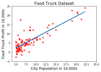
Now let’s use this function to train our model and plot the hypothesis function:
1 | theta = gradient_descent(X, y, 0.02, 600) # run GD for 600 iterations with learning rate = 0.02 |
Debugging
Our linear fit looks pretty good, right? The algorithm must have successfully optimized our model.
Well, to be honest, it’s been fairly easy to visualize the hypothesis because there’s only one feature in this problem.
But what if we had multiple features? Then it wouldn’t be possible to simply plot the hypothesis to see whether the algorithm has worked as intended or not.
Fortunately, there’s a simple way to debug the gradient descent algorithm irrespective of the number of features:
- Modify the gradient descent function to make it record the cost at the end of each iteration.
- Plot the cost history after the gradient descent has finished.
- Pat yourself on the back if you see that the cost has monotonically decreased over time.
Here’s the modified version of our gradient descent function:
1 | def gradient_descent(X, y, alpha, num_iters): |
Now let’s try learning rates $0.01$, $0.015$, $0.02$ and plot the cost history for each one:
1 | plt.figure() |
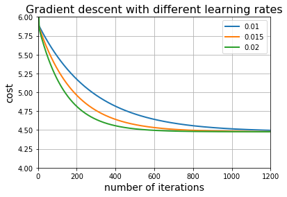
It appears that the gradient descent algorithm worked correctly for these particular learning rates. Notice that it takes more iterations to minimize the cost as the learning rate decreases.
Now let’s try a larger learning rate and see what happens:
1 | learning_rate = 0.025 |
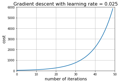
Doesn't look good... That's what happens when the learning rate is too large. Even though the gradient descent algorithm takes steps in the correct direction, these steps are so huge that it's going to overshoot the target and the cost diverges from the minimum value instead of converging to it.
Right now we can safely set the learning rate to $0.02$, because it allows us to minimize the cost and it requires relatively fewer iterations to converge.
Prediction
Now that we’ve learned how to train our model, we can finally predict the food truck profit for a particular city:
1 | theta, _ = gradient_descent(X, y, 0.02, 600) # train the model |
For population = 70,000, we predict a profit of $ 45905.6621788If you’re still here, you should subscribe to get updates on my future articles.