One-vs-All Classification
First of all, let me briefly explain the idea behind one-vs-all classification. Say we have a classification problem and there are $N$ distinct classes. In this case, we’ll have to train a multi-class classifier instead of a binary one.
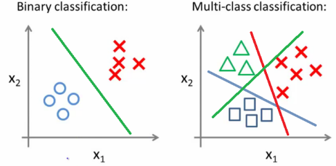
One-vs-all classification is a method which involves training $N$ distinct binary classifiers, each designed for recognizing a particular class. Then those $N$ classifiers are collectively used for multi-class classification as demonstrated below:

We already know from the previous post how to train a binary classifier using logistic regression. So the only thing we have to do now really is to train $N$ binary classifiers instead of just one. And that’s pretty much it.
Problem & Dataset
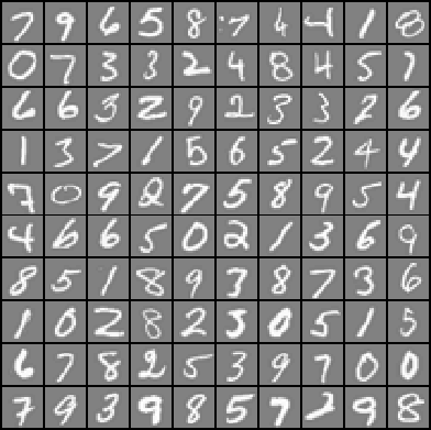
We’re going to use this one-vs-all approach to solve a multi-class classification problem from the machine learning course thought by Andrew Ng. The goal in this problem is to identify digits from 0 to 9 by looking at 20x20 pixel drawings.
Here the number of classes $N$ is equal to 10, which is the number of different digits. We’re going to treat each pixel as an individual feature, which adds up to 400 features per image. Here are some examples from our training sample of 5000 images:

The training data is stored in a file called digits.mat. The reason that it’s a .mat file is because this problem is originally a Matlab assignment. No big deal, since it’s pretty easy to import a .mat file in Python using the loadmat function from the scipy.io module. Here’s how to do it:
1 | import numpy as np |
Let me point out two things here:
We’re using the
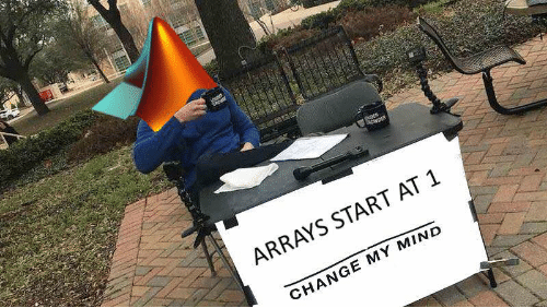
squeezefunction on theyarray in order to explicitly make it one dimensional. We’re doing this becauseyis stored as a 2D matrix in the.matfile although it’s actually a 1D array.We’re replacing the label 10 with 0. This label actually stands for the digit 0 but it was converted to 10 because of array indexing issues in Matlab.

Logistic Regression Recap
Remember the sigmoid, cost and cost_gradient functions that we’ve come up with while training a logistic regression model in the previous post? Here we can reuse these functions exactly as they are, because we’re going to train nothing but logistic regression models also in this problem.
1 | def sigmoid(z): |
Training Stage
The final thing we have to do before starting to train our multi-class classifier is to add an initial column of ones to our feature matrix to take into account the intercept term:
1 | X = np.ones(shape=(x.shape[0], x.shape[1] + 1)) |
Now we’re ready to train our classifiers. Let’s create an array to store the model parameters $\theta$ for each classifier. Note that we need 10 sets of model parameters, each consisting of 401 parameters including the intercept term:
1 | classifiers = np.zeros(shape=(numLabels, numFeatures + 1)) |
Then we’re going to train 10 binary classifiers targeted for each digit inside a for loop:
1 | for c in range(0, numLabels): |
Here we create a label vector in each iteration. We set its values to 1 where the corresponding values in y are equal to the current digit, and we set the rest of its values to 0. Hence the label vector acts as the target variable vector y of the binary classifier that we train for the current digit.
Predictions
We can evaluate the probability estimations of our optimized model for each class as follows:
1 | classProbabilities = sigmoid(X @ classifiers.transpose()) |
This will give us a matrix of 5000 rows and 10 columns, where the columns correspond to the estimated class (digit) probabilities for all 5000 images.
However, we may need the final predictions of the optimized classifier instead of numerical probability estimations. We can find out our model’s predictions by simply selecting the label with the highest probability in each row :
1 | predictions = classProbabilities.argmax(axis=1) |
Now we have our model’s predictions as a vector with 5000 elements labeled from 0 to 9.
Accuracy
Finally, we can compute our model’s training accuracy by computing the percentage of successful predictions:
1 | print("Training accuracy:", str(100 * np.mean(predictions == y)) + "%") |
Training accuracy: 94.54%An accuracy of 94.5% isn’t bad at all considering we have 10 classes and a very large number of features. Still, we could do even better if we decided to use a nonlinear model such as a neural network.
If you’re still here, you should subscribe to get updates on my future articles.